4 Statistical Genetics

4.1 Phasing

We use WhatsHap to phase genotypes in a pedigree using the Mendelian transmission rules and physical phasing based on reads that span two or more heterozygous variants.

whatshap phase --ped pedigree.ped \
-o phased_whatshap.vcf joint/output_vqsr_variants.vcf.gz \
aligned_HG002.bam aligned_HG003.bam aligned_HG004.bam \
--tag=PS --no-reference --indels

4.2 Kinship

We seek to verify pedigree relationships and identify hidden relatedness between samples. We first select SNPs in approximate linkage equilibrium with Linkdatagen based on the genetic linkage map of HapMap SNPs. Linkdatagen also eliminates Mendelian inconsitencies in the data.

# Split variant calling file into seperate files for each individual
bcftools +split AJ_output_vqsr_snps_hard_indels.vcf.gz -Ov -o split

# Write path to each individual's vcf in a text file named MyVCFlist.txt
perl vcf2linkdatagen.pl \
-variantCaller unifiedgenotyper \
-annotfile annotHapMap2U_hg38.txt \
-pop CEU -mindepth 10 -missingness 0 \
-idlist MyVCFlist.txt > HG002_trio.brlmm

perl linkdatagen.pl \
-data m -pedfile MyPed.ped \
-whichSamplesFile MyWS.ws \
-callFile MySNPs.brlmm \
-annotFile annotHapMap2U.txt \
-pop CEU -binsize 0.3 \
-MendelErrors removeSNPs -prog pl \
-outputDir MyPed_HapMap2_pl > MyPed_HapMap2_pl.out

We construct an allele frequency report for the chosen SNPs.

library(tidyverse)
map <- read_delim(file = "data/plink.map", delim = " ", col_select = 1:4, col_names = c("CHR", "SNP", "cM", "bp"))
ord <- read_tsv(file = "data/orderedSNPs.txt")
freq_pl <- map %>% left_join(ord, by = "SNP") %>% 
  dplyr::select(CHR, SNP, `Allele freq`) %>% 
  mutate(A1="1") %>% mutate(A2="2") %>% mutate(NCHROBS="300") %>% 
  dplyr::select(CHR, SNP, A1, A2, `Allele freq`, NCHROBS) %>% 
  dplyr::rename(MAF = `Allele freq`)
write_delim(freq_pl, "result/freq_pl.frq", delim = " ")

Alternatively, with a sufficient number of samples, we can estimate the linkage disequilibrium between alleles and remove correlated SNPs using PLINK.

plink --file data --indep 50 5 2

We then calculate the empirical kinship coefficient by estimating identity by descent based on identity by state and population allele frequencies (Lange 2002). We run this calculation in PLINK.

module load plink/1.9b_6.21-x86_64
plink --file plink --genome full --read-freq freq_pl.frq

We also run this calculation using MendelKinship from the OpenMendel project.

using MendelKinship, CSV
Kinship("control_compare.txt")

We obtain the following results for the AJ reference trio using PLINK. PI_HAT is two times the estimated kinship coefficient between individuals IID1 and IID2. We note that the estimated kinship coefficient between individuals HG003 and HG004, which equals the the inbreeding coefficient of their son HG002, is 0.

IID1	IID2	RT	EZ	Z0	Z1	Z2	PI_HAT	DST	IBS0	IBS1	IBS2
HG002	HG003	PO	0.5	0	1	0	0.5	0.752334	0	2918	2973
HG002	HG004	PO	0.5	0	1	0	0.5	0.756153	0	2873	3018
HG003	HG004	OT	0	1	0	0	0	0.616449	638	3243	2010

4.3 Runs of Homozygosity

If we suspect some degree of consanguinity, we may look for a homozygous pathogenic variant in runs of homozygosity using AutozygosityMapper.

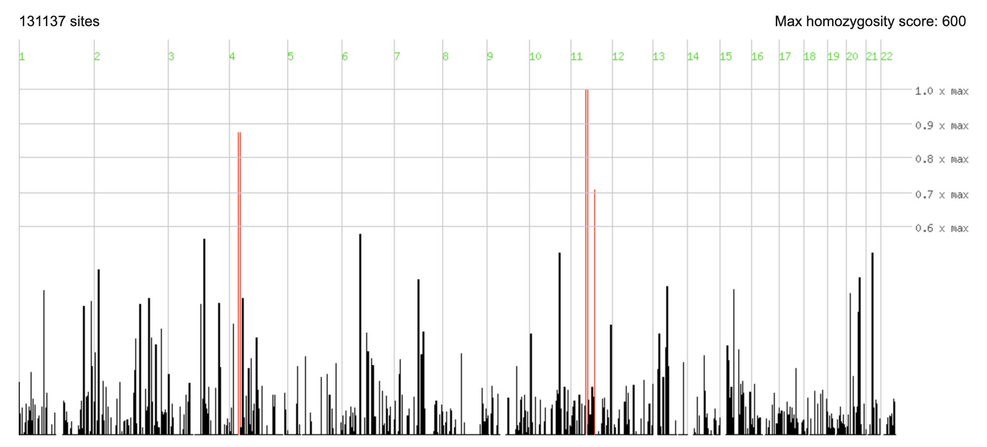
AutozygosityMapper report for HG002 as case and HG003 and HG004 as controls.

4.4 Linkage Analysis

Using the same set of SNPs in linkage equillibrium, we can run linkage analysis on appropriately chosen pedigrees using OpenMendel for two-point linkage or multipoint linkage analysis.

# Two-point linkage analysis
using MendelTwoPointLinkage, CSV
TwoPointLinkage("Control_file.txt")

# Multipoint linkage analysis
using MendelLocationScores, CSV
LocationScores("Control_file.txt")

4.5 Population Substructure

Given a large number of samples from a population, we cluster individuals by degree of identity by state using PLINK in order to identify subgroups with shared ancestry.

plink --file mydata --cluster
# dimensional reduction to 4D then plot two coordinates
plink --file mydata --read-genome plink.genome --cluster --mds-plot 4